
How to use
Please prepare your own Excel.
the questions are japason’s original.
MO-210:Pass With 91 Questions
if you can solve all the questions in this video, you will definitely pass the exam.
Chapter1: Manage Worksheets and Workbook
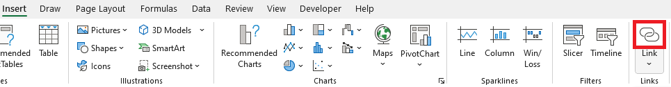
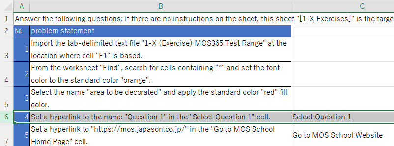
Insert and remove hyperlinks
Q1. Set a hyperlink to “https://mos.japason.co.jp/” in A1 cell.
answer
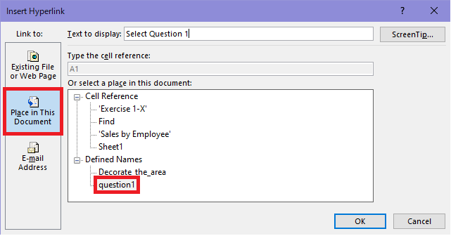
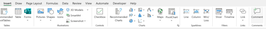
- Select A1 cell, and click on the “Insert” tab – “Link” icon.
- From “Place In This Document,” select “question1” in “Defined Names” and click “OK”.
Navigate to named cells, ranges, or workbook elements
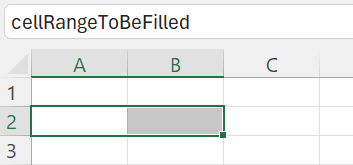
Q2.Define the name “cellRangeToBeFilled” for A2:B2.
answer
- select A2:B2, and enter cellRangeToBeFilled in namebox.
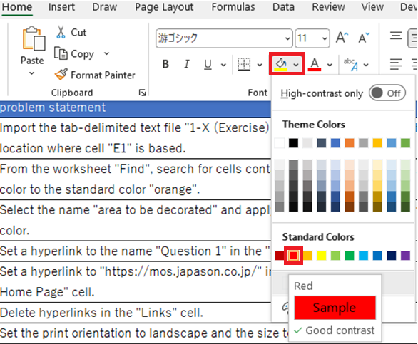
Q3.Select the named range ” cellRangeToBeFilled” and apply the standard color “red” fill color.
answer
- Press Ctrl+G to open the “Jump” window, select “cellRangeToBeFilled” and press “OK”.
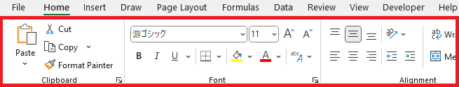
- On the Home tab, in the Font group, select Fill Color – Red.
Format worksheets and workbooks
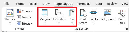
Q4.Change the orientation to landscape and the size to A3.
answer
- Select “Page Layout” tab – “Orientation” – “Landscape”

2. Select “Page Layout” tab – “Size” – “A3
Q5.Change the margins to wide.
answer
- Page Layout tab – Margins – Wide
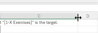
Q6.Enter “I like this.” in Cell C1, andAutomatically adjusts the width of column C.
answer
- (Enter “I like this.” in Cell C1)
- Place the pointer to the right side of column C and double-click
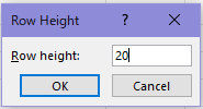
Q7.Set the height of the 12th row to exactly “20”.
answer
Right-click on line 12 -〈Row Height〉.
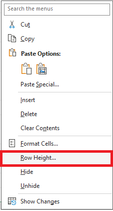
- Copy and paste “20” from the question text and press [OK].
Q8.Display the sheet name in the center of the header. When finished, return to Normal view.
answer
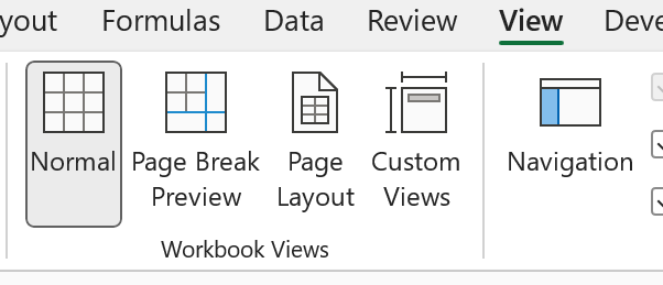
- On the View tab, select Page Layout.
- Click on the center of the header.
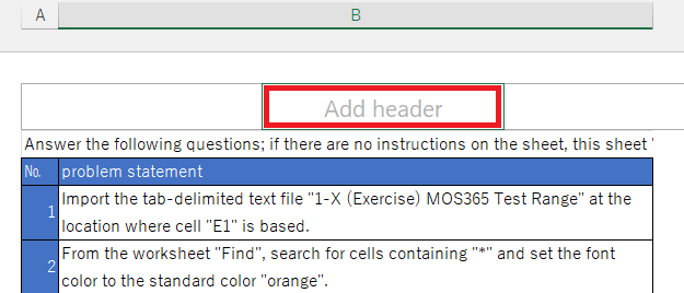
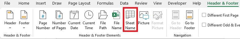
- Select the “Header & Footer” tab – “Sheet Name”.
- Click on anything other than the header/footer to stop the edit mode of header/footer.
- From the View tab, select Normal.
customize options and views
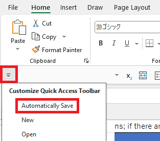
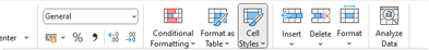
Q9.Add Auto Save to the Quick Access Toolbar.
answer
Right-click on the ribbon – Show Quick Access Toolbar
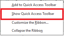
In the “Quick Access Toolbar”, click on the Down Arrow and select Automatically Save.
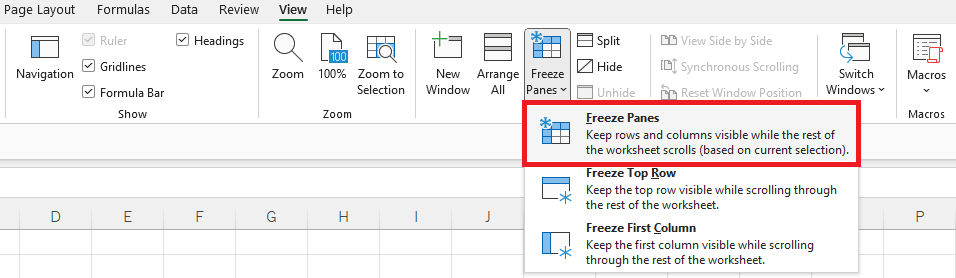
Q10.Configure the rows 1 through 5 remain visible as you scroll vertically.
answer
- Select line 6.
2.Select View tab – Freeze Panes
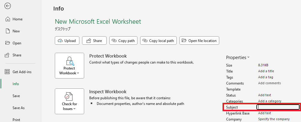
Q11.Add the value “Chapter1Exercises” to the subject property of the book document.
answer
Click on the “File” tab, then select Info,and then select “Show All Properties”.
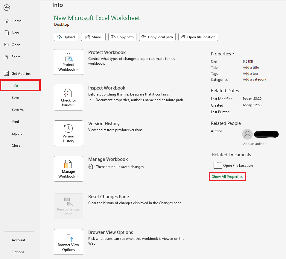
- On the subject, copy and paste “Chapter1Exercises” from the question text.
Prepare workbooks for collaboration and distribution
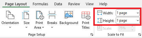
Q12.Configure print settings to fit on a singe page when printed.
answer
In the Page Layout tab-Scale to Fit, specify1 page for Width and Height respectively.
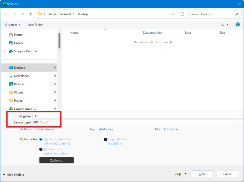
Q13.Save the “Chapter1Exercises” worksheet into your desktop as a PDF file with the name “PDF”.
*In the exam, a folder is pre-created but this time prepare and Excel data that you are saving in advance.
answer
1.Create the “MOS365” folder on your desktop.
2.Back to the Excel and press F12 to launch the “Save As” window.
3.Select “MOS365” folder on the desktop and enter “PDF” as the file name (copy and paste from the question text).
4.Select “PDF” for “Save as type” and click “Save”.
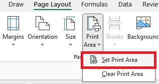
Q14.Set cells A2:B10 so they will be the only cells that print.
answer
1.Select A2:B10.
2.Page Layout tab -PrintArea -Set Print Area.
Manage Comments
(Advance preparation)
Add a comment to the cell B4 and write “Please confirm” .
1.Select the B4 cell and go to Insert tab -Comment – Comment.
2.Copy and paste “Please confirm” from the B4 cell and then click the Airplane button.

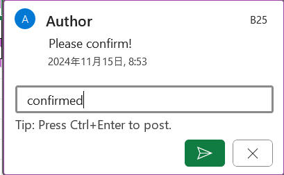
Q15.Reply to the comments in this cell with “confirmed” .
answer
1.Right-click on the B4 cell in question and show the Comment.
2.Type “confirmed” in the reply box (copy and paste from the question text), and then click the “paper airplane” button.
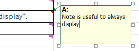
Q16.Add a note to this cell and write “Note is useful to always display”.
answer
1.Copy “Note is useful to always display” from the question text.
2.Right-click on a cell and select “New Note” from the menu.
3.Paste “Note is useful to always display” .
Chapter2: Manage Data Cells and Ranges
MO-210:Pass With 91 Questions
if you can solve all the questions in this video, you will definitely pass the exam.
Manipulate data in worksheets
(Advance preparation)
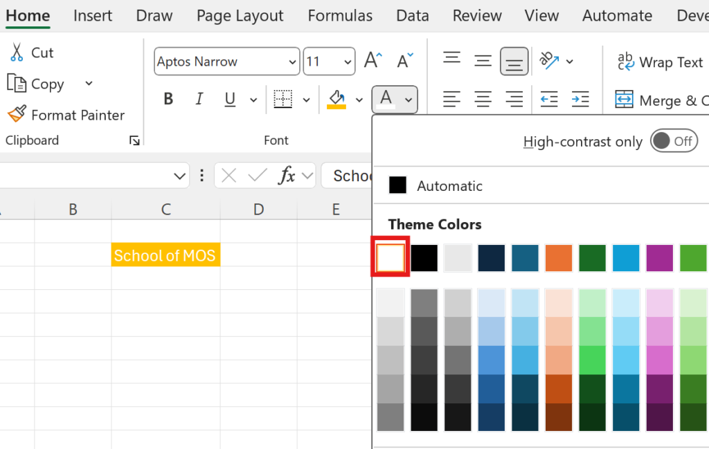
1.Type “School of MOS” into the cell C2 and then, apply orange color from Home tab-Fill Standard color-Orange.
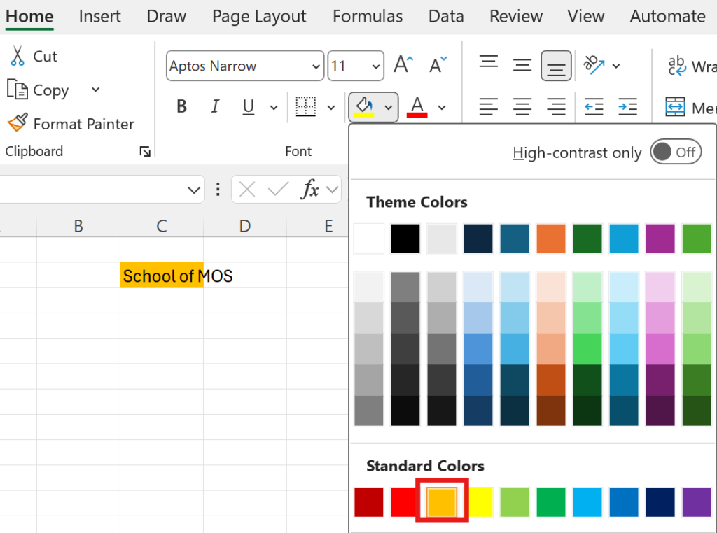
2.On the Home tab, in the Font group, click Font Colors, and select Whiite.
Q17.Copy cell C2 and paste only the value into cell D2.
answer
1.Select cell C2 and press Ctrl+C
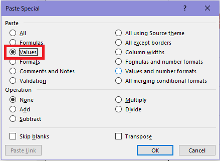
2.Select cell D2, then press Ctrl+Alt+V to launch the <Paste Special> window.
3.Select [Values] and press [OK].
(Advance preparation)
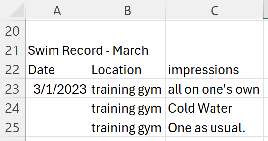
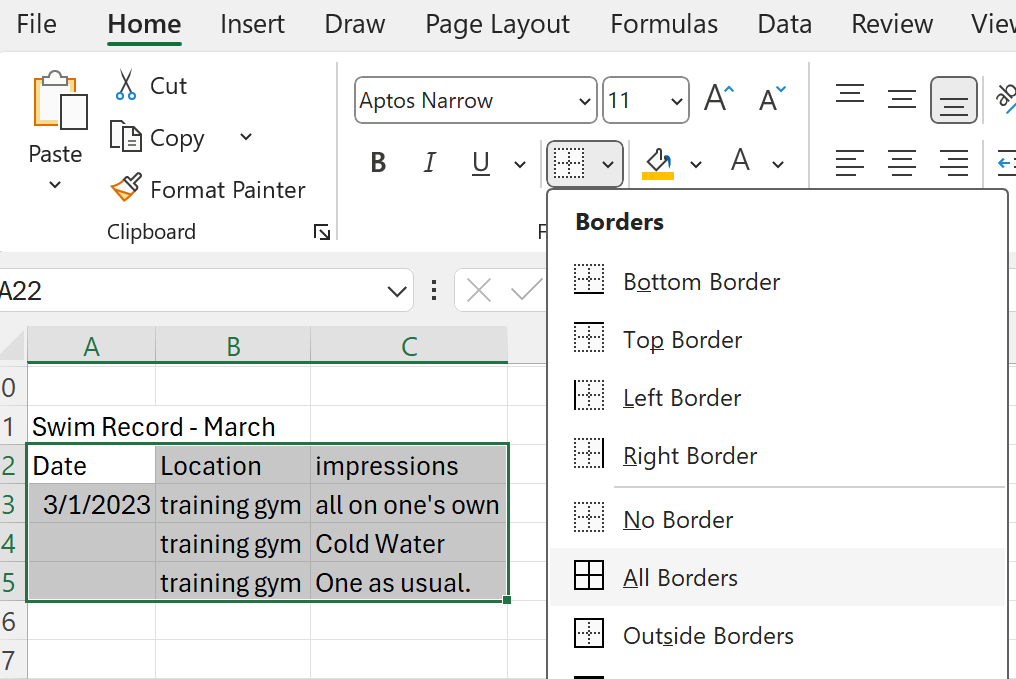
Create the table on A21:C25 as below.
1.Enter the text and value into A21:C25.
2.Select A22:C25 and right-click and select Borders – All Borders.
7.Select B24:C24 and right-click to select insert.
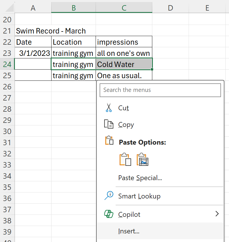
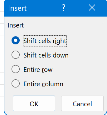
8. Select Shift right and click OK button.
Q18.Use Auto Fill to fill the date columns of the “Swim Records March” table”.
answer
1.Select the A23 cell and place the mouse pointer over the lower right corner of the cell to display a crosshair.
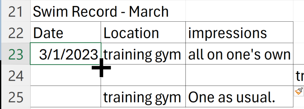
2.Double-click (or drag to cell A25)
Q19. Delete the blank cells in the “Swim Records – March” table to make the table more complete.
answer
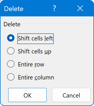
1.Select and right-click on a blank cell (the two cells to the right of 2023/3/2) in the “Swim Records – March” table.
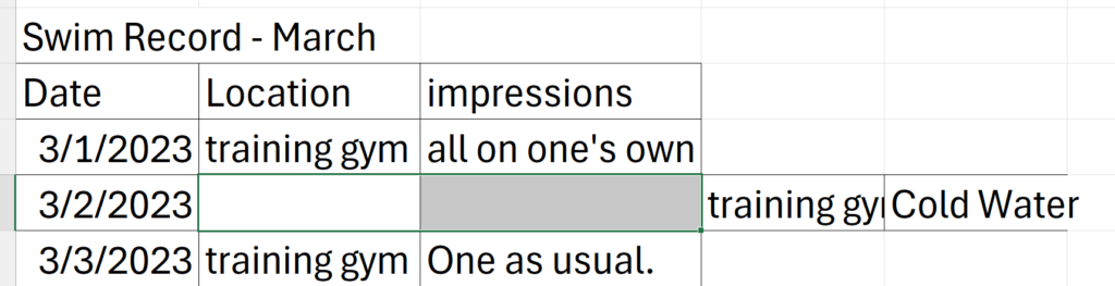
2.click delete
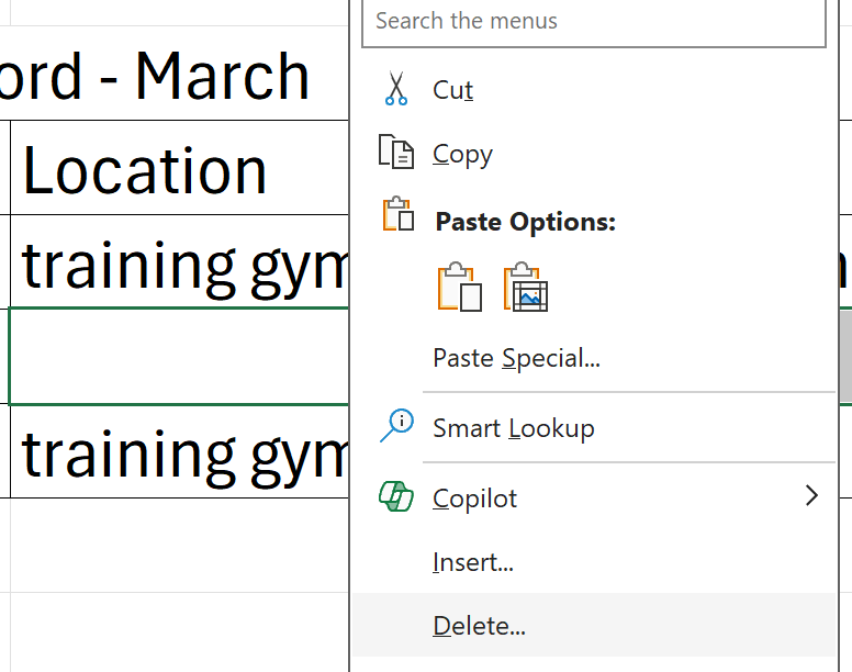
3.Confirm that the shift cells left is selected, and press [OK].
Format cells and ranges
(Advance preparation)
1.Type “Merge it” into the cell C5 .
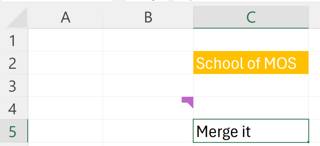
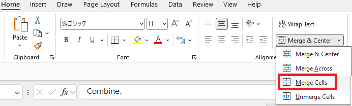
Q19.Merge cells C5:D5 without changing the alignment of the contents.
answer
1.Select C5:D5 and click Home tab-Alignment–”v”to the right of the Merge & Center.
2.Select “Merge Cells”.
(Advance preparation)
1.Type “Almost halfway” into the cell C7 .
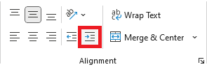
Q20.Set the left indent of the texts in the cell C7 to 2 characters.
answer
1.Select C7, and click “Home”tab-“Alignment”-“Increase Indent”(the one with the→symbol) twice.
(Advance preparation)
1.Type “School of MOS” into the cell C2 and then, apply orange color from Home-tab-Fill color-Standard color-Orange.
2.On the Home tab, in the Font group, click Font Colors, and select White.
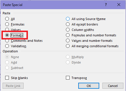
Q21.Apply the formatting of cell C2 to cell A1.
answer
1.Select cell C2 and press Ctrl+C
2.Select cell A1, then press Ctrl+Alt+V to launch the <Paste Special> window.
3.[Formats] and press [OK]
(Advance preparation)
1.Type “Three chapters left after this question” into the cell C9 .
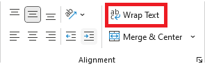
Q22.Wrap the string in cell C9.
answer
1.Select cell C9 and click on the “Home” tab-“Alignment”-“Wrap Text”.
(Advance preparation)
1.Type 100 into the cell C10.
Q23.Display cell C13 to three decimal places.
answer
1.Select cell C10, and click Home tab-Number-Increase Decimal (the one with the←symbol) three times.
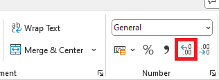
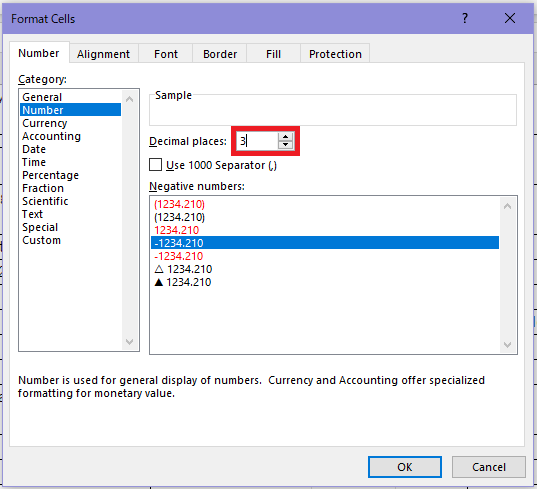
(Another solution)
1.Select cell C10 and click the down-right arrow in the”Number” group to open the “Format Cells” window.

2.Enter “3” for decimal places.
(Advance preparation)
Type “3/14” into the cell C11.
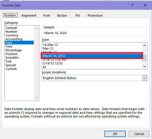
Q24.Display the date in cell C13 in the format “March14,2023”
answer
1.Select the cell C11 and from the Home tab, click the down arrow to the right of the number to launch the cell formatting window.
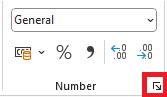
2.Select <March14, 2023> from the display format and click”OK”.
(Advance preparation)
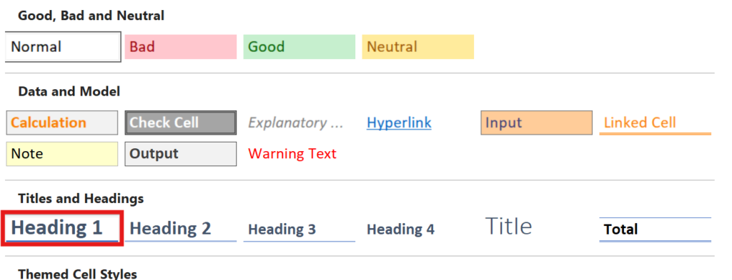
Type “Heading 1” into the cell C12.
Q25.Apply the”Heading 1″style to cellC12.
answer
1.SelectC12, then select Home tab-Style-Cell Styles-Heading 1.
(Advance preparation)
1.Type “White” into the cell C13 and select Blue color from Home tab-Fill Color-Theme Color.
2.Set the font color in White from Font-Theme Color.
3.Apply Bold font.
Q26.Clear the formatting in cell C13.
answer
1.Select cells with no formatting or values entered and press Ctrl+C to copy it.
2.Select C13, then press Ctrl+Alt+V to launch the Paste Special window
3.Select “Formats” and click “OK”.
Define a named range
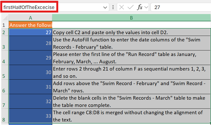
Q27.Define the name “FirstHalfOfTheExcecise” in cells A2:B8.
answer
1.Select cells A2:B8
2.In the name box, type “FirstHalfOfTheExcecise”(copy and paste from the question text) and press Enter key to confirm.
Summarize data visually
(Advance preparation)
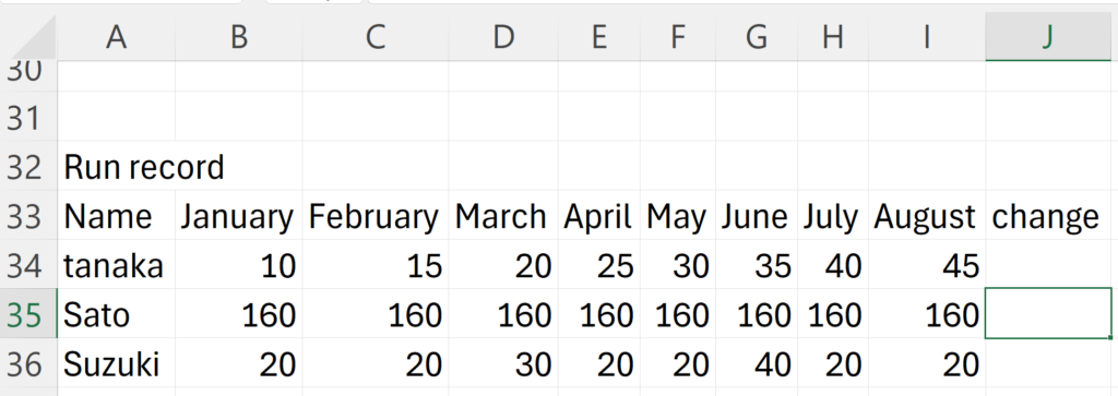
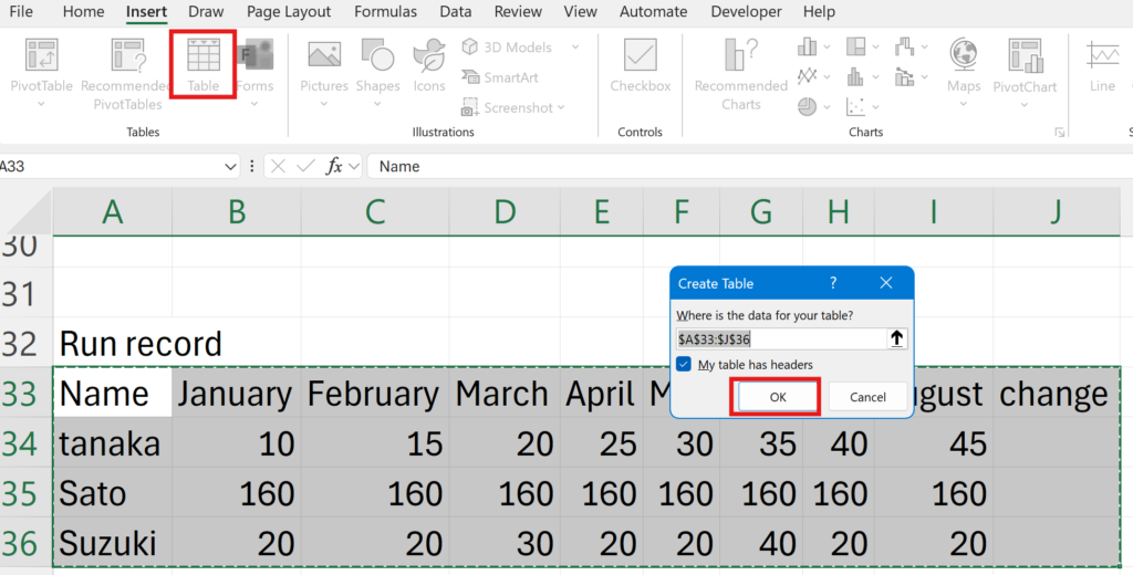
Create the table”Run Record”.
1.Type the texts and value on the A33:J36 as below.
2.Select A33:J36 and click Insert tab-Table-OK.
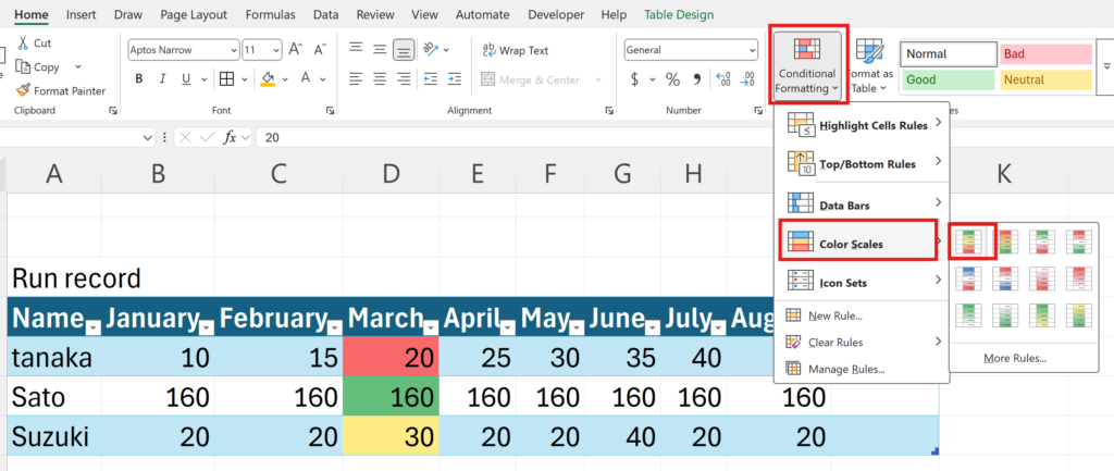
3.Select D34:D36 and click Home tab-Style-Conditional Format-Color Scale-Green Yellow Red color scale.
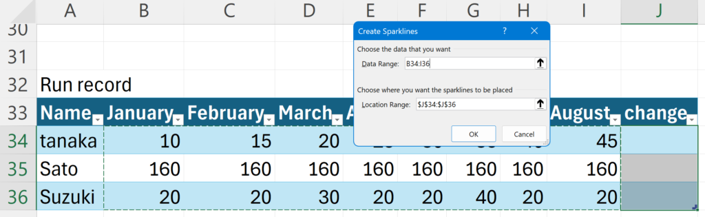
Q28.Based on the values in the table”Run Record”, insert a column spark line in the “change” column.
answer
1.Select cells of change column J34:J36.
2.Insert tab-“Sparklines”-Column
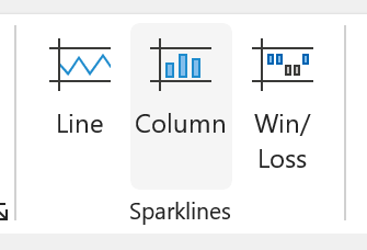
3.Select the range of cells B35:I37 and click “OK”.
Q29.For the August column of the table”Run record”, format the cells smaller than 50 with”Light red Fill with Dark red Text”.
answer
1.Select the cell I34:I36 and click Home tab-Conditional Formatting–HighlightCellRules–”Less than…”.
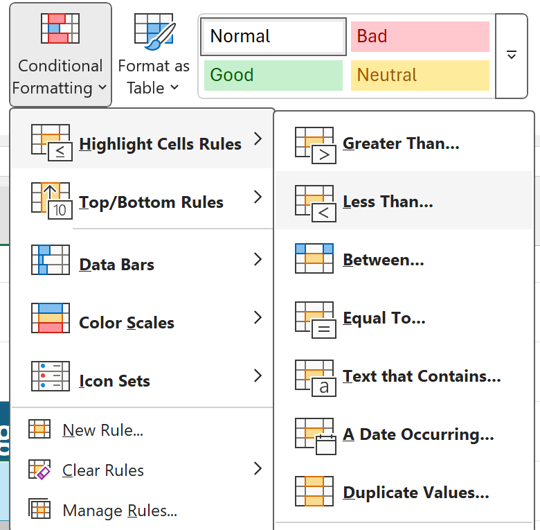
2.Copy and paste “50” from the question text into “Format cells that are Less Than” and click “OK”.
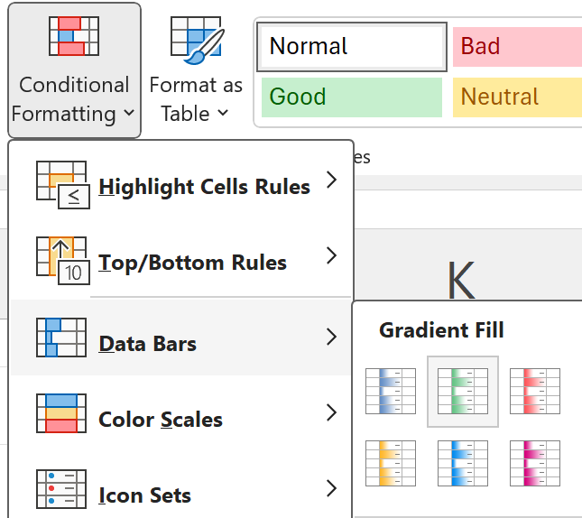
Q30.Display the green gradient data bar in the January column of the table “Run record”.
answer
1.Select the January column and choose “Green Data Bar” in the Home tab-Conditional Formatting-Data Bar–GradientFill
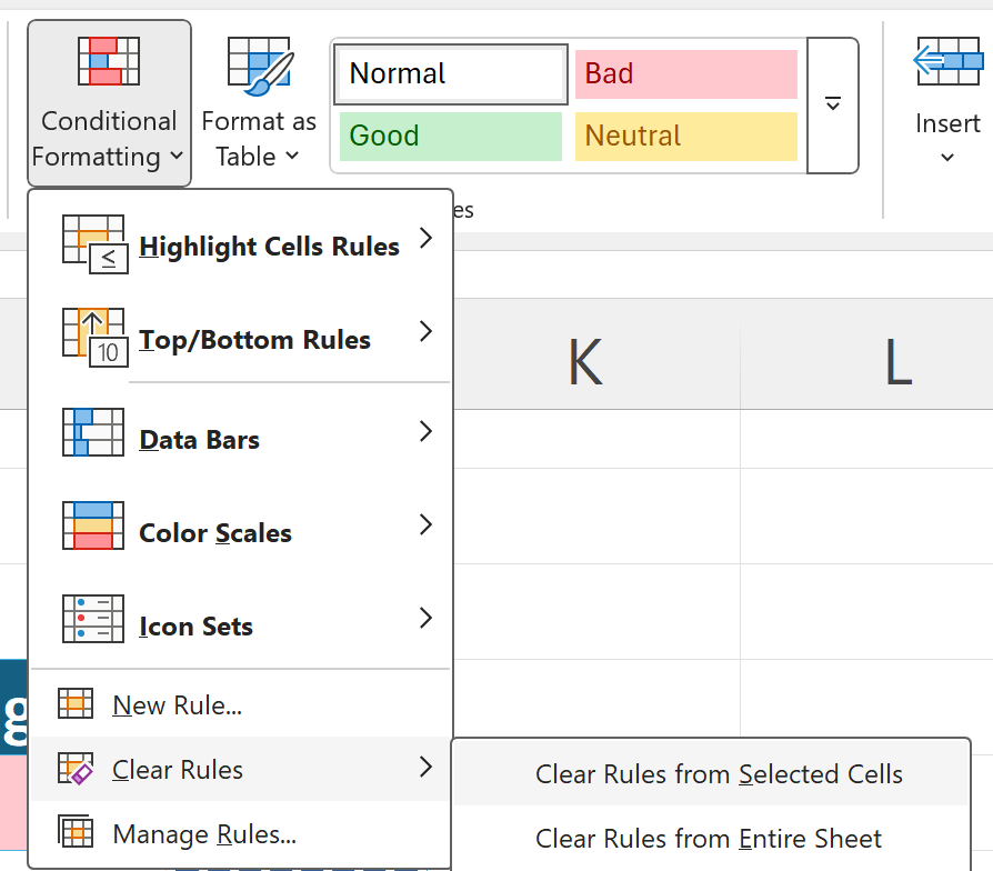
Q31.Remove the conditional formatting set in the March column of the table “Run Records”
answer
1.Select the March column, then select the Home tab-Conditional Formatting-Clear Rules-Clear Rules from Selected Cells.
Chapter 3: Manage Tables and Table Data
MO-210:Pass With 91 Questions
if you can solve all the questions in this video, you will definitely pass the exam.
Create and format tables
(Advance preparation)
Create the table as below.
1.Type the texts below into A1:E5.
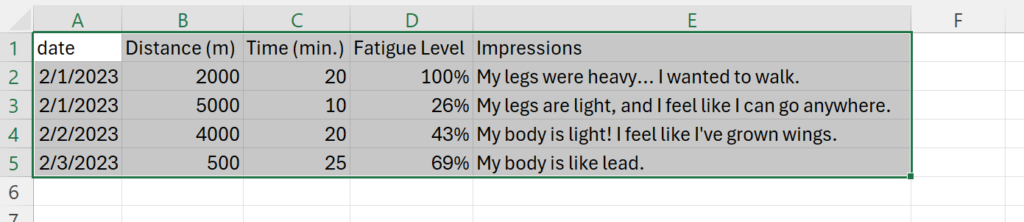
Q32.Change cell range A1:E5 to a table; the first row is used as the title.
answer
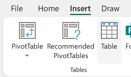
1.Select A1:E5 and click on Insert tab-Tables-Table.
2.Make sure that “My table has headers” is checked, and click”OK.
Q33. Apply style “Gold, Table Style Midium 5” to table A1:E5.
answer
1.Click on a cell in the table you created.
2.Table Design tab-Select “Gold, Table Style Midium 5
Modify tables
Q34.Add column “Weather” to table A1:E5, to the left of Distance (m), so that nothing but the table is affected.
answer
1.Select the distance column in the table and right-click-Insert-Table Columns to the left.
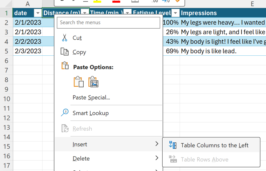
2.Press Ctrl+C “Weather” in the question to copy and press Ctrl+V to paste into the column 1.
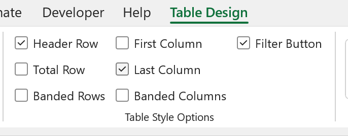
Q35.Remove stripes from table A1:E5 and highlight the last column.
answer
1.Click on a created cell in the table.
2.From the Table Design tab-Table Style Options, uncheck Banded Rows and check Last column .
Q36.Display the total rows in table A1:E5, showing the total for Distance (m) and Time (min), and the average for Fatigue Level. Not display for Comments.
answer
1.Click on a created cell in the table.
2.From the Table Design tab-Table Style Options, check Total Row.
3.As instructed in the question text, select the item for each row. Select “None” for the “Impressions” row.
Q37.Sort the table A1:E5 in descending order of Time(min); if Time (min)s are the same, then in ascending order of Fatigue Level.
answer
1.Click[▼] on one of the table headings and choose Sort by Color-CustomSort… to open the Sort window.
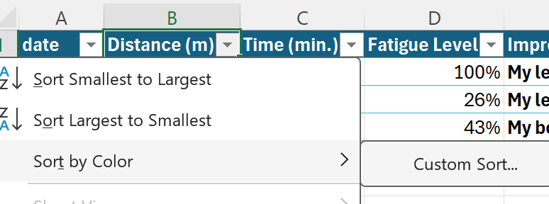
2.Specify Time(min.) for the column and Largest to Smallest for the order.
3.Click Add level, specify the columns FatigueLevel, and click OK.
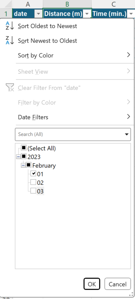
Q38.A1:E5 table should show only records for the day of Feb 1. do not delete data.
answer
1.Click [▼] under the heading “date” and uncheck “02” and “03” and click [OK].
(Advance preparation)
Create the table “Student List”.
1.Type texts and value in the cell A7:B10 as below.
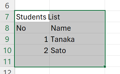
2.Select A8:B10 and click insert tab-table then press ok.
Q39.Display only records from the “Student List” table whose name begins with”Ta”.
answer
1.Click [▼] inthe heading”Name”and select Text Filters-Begins With…
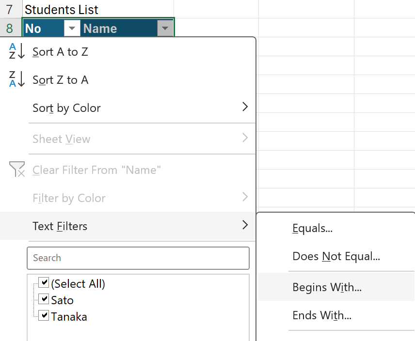
2.Enter”Ta”in the first text box (copy and paste from the question text), and click “OK”.
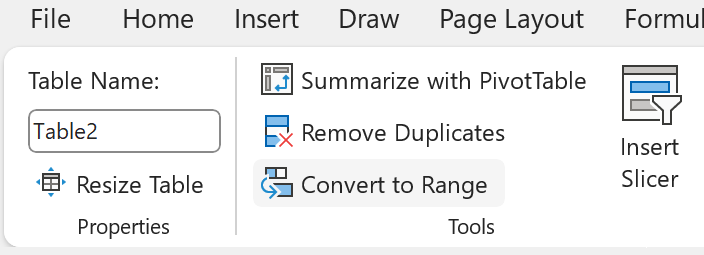
Q40. Remove the table formatting from the “Student List”.
answer
1.Click on a cell in the table.
2.Click on Table Design tab-“Convert to Range”
Chapter4: Perform Operations by using Formulas and Functions
MO-210:Pass With 91 Questions
if you can solve all the questions in this video, you will definitely pass the exam.
Insert references
(Advance preparation)
Create the table in the cell A1:E6.
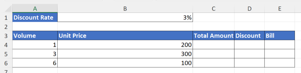
Q41.In the Total Amount column, enter the formula to multiply the volume by the unit price to obtain the amount.
answer
1.Enter “=” in the cell B3 C4.
2.Click on cell A4(or enter the left arrow twice).
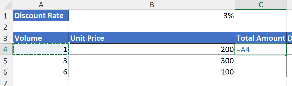
3.Next, enter”*”(asterisk).
Then, click cell B4(or or enter the left arrow once) and press Enter key.
4.Copy formulas to C5:C6 using the Auto Fill function.(Copy & Paste is also OK. Likewise hereafter.)
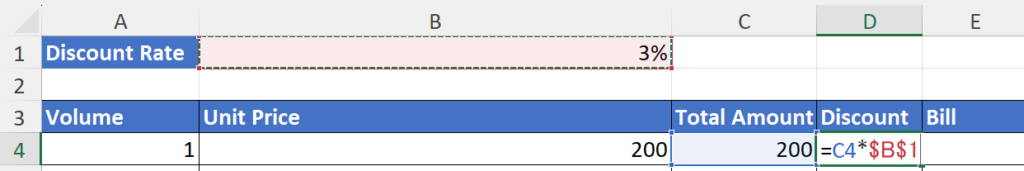
Q42.In the Discount column, enter the formula to determine the discount amount, which is calculated by multiplying the total amount by the discount rate in cell B1.
answer
1.Enter “=C4*” in cell D4
2.Select cell B1, press the F4 key once to make it an absolute reference (with the$ symbol in two places before B and 1) and confirm with Enter key.
Q43.In the Bill column, enter the formula to find the total amount minus the discount.
answer
1.Enter”=C4-D4″in cell E4.
2.Copy formulas to the cell below.
Calculate and transform data 1
(Advance preparation)
Create the table as below.
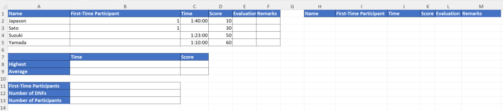
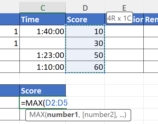
Q44.Enter the highest score using the MAX function in cell C8.
answer
1.Enter”=max”in cell C8.
2.With “MAX” selected from the suggestion list, press theTab key.
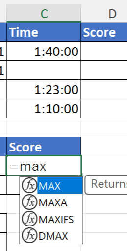
3.Select the range D2:D5 and press Enter key to confirm.
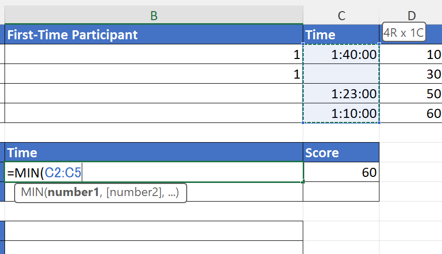
Q45.Use the function to display the best record in B8. The best record refers to the fastest time.
answer
1.Enter”=MIN(C2:C5)”in cell D8.
Q46.Use the function to display the average time in cell B9.
answer
1.Enter”=AVERAGE(C2:C5)”in cell B9
Q47.Use the function to display “failed” in cell B11 for those scoring nothing.
answer
1.Enter “=COUNTBLANK(C2:C5)” in cell B11.
Q48.Use the function to display he number of participants in cell B12. Count the name cells.
answer
1.Enter “=COUNTA(A2:A5)” in cell B12.
Q49.Use the function to indicate”Beginner”if the first time participant column has the value”1″, otherwise, indicate “Experienced”in the Remarks column.
answer
1.Enter “=IF(” in the cell F2.
2.Press FX button to launch the function argument window and enter the following.
Click on cell B2 and enter”=1″
Enter Beginner inValue_if_true.
Enter Experienced in the Value_if_false field.
3.Copy formulas to the cells below.
Q50.Use the function to display”failed”in the evaluation column for those scoring less than 50 points and if otherwise, nothing.
answer
1.Type “=IF” in cell E2, select “IF” from the suggestion list
2.Press the “FX” button to open the “Function Arguments” window and enter the following.
Click on cell D2 and enter”<50″
Enter”failed”forValue_if_true.
Enter””forValue_if_false
3.Copy formulas to the cells below.
Q51.Use the function to sort the table in descending order of scores, with H2 as the base point.
answer
1.Enter”=sort”in cell H2.
2.Press the”FX”button to open the”Function Arguments”window an enter the following.
Array A2:F5
Sort_index 4
Sort_order -1
Format and modify text
(Advance preparation)
Create the table.
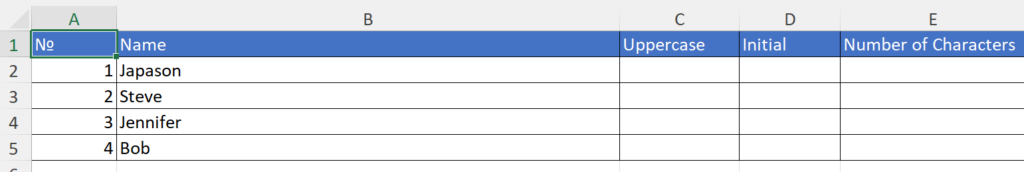
Q52.Use function to convert the name in column B to uppercase in the “uppercase” column.
answer
1.Enter “=UPPER(B2)” in the cell B2.
2.Auto-fill downward.
Q53.On the sheet 3, Use the function to display the first letter of the names in the initial column.
answer
1.Type”=LEFT(B2,1)” in the cell D2.
2.Auto-fill downward.
Q54.Use the functions to join the “No” and “Name” columns in the “Player’sNumber ” They should bejoined by a “-“.
answer
1.Enter “=TEXTJOIN(” in the cell E2.
2.Press FX button and enter the following.
Delimiter “-“
Text 1 A2
Text 2 B2
3.Auto-fill downward.
Calculate and transform data 2
(Advance preparation)
Create the table.
selecet B3:B12 and define the name “ParticipantsName”
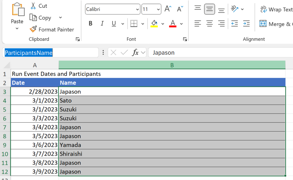
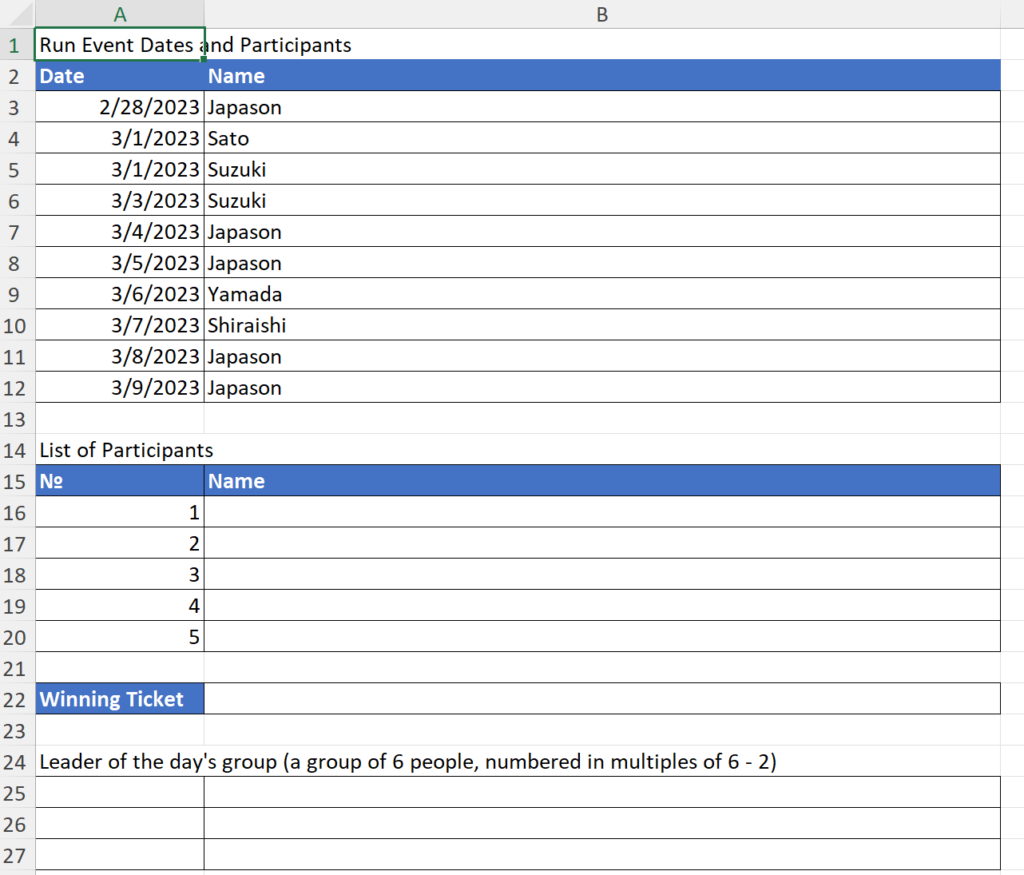
Q55.Use the function to display the data from the”Name”column of the table “RunEvent Dates and Participants” with duplicates eliminated, starting at cell B16. In the formula, use the defined name.
answer
1.Enter”=uni”incell B16, select<UNIQUE>from thesuggestionsand presstheTab key.
2.Select<ParticipantsName>from the list of suggestions and press Enter.
Q56.On the sheet 4,Use the function to display a random value within the range of1 to 5 in cell B22.
answer
1.Enter “=RANDBETWEEN(1,5)” in the cell B22.
Q57.Use theFunction to display numerical data in three rows and two columns starting atcell A25 with the number biginning from1.
answer
1.Enter “=SEQUENCE(3,2)” in cell B25.
Q58.Display the formulas on this sheet.
answer
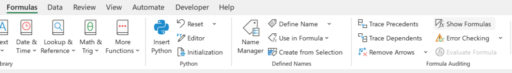
1.On the”Formulas”tab-Click onShow Formulas.
Chapter 5: Manage Charts
MO-210:Pass With 91 Questions
if you can solve all the questions in this video, you will definitely pass the exam.
(Advance preparation)
Create the below table.
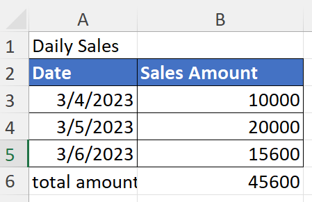
Q59.Create a clustered column chart using the Daily Sales table.
answer
1.Select everything except for the totalfrom theDaily Sales table.
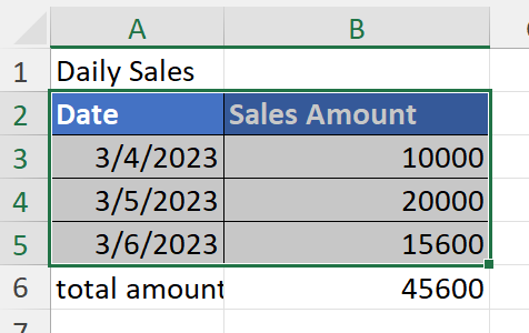
2.Insert tab-click on “RecommendedCharts” in Charts.
3.Select “ClusteredColumn” and click “OK”.
(Advance preparation)
Use the DailySales table to create the below pie chart.
1.Select everything except for the total from the Daily Sales table.
2.Insert tab-click on”Recommended Charts” in Charts.
3.Select “Pie Chart” and click”OK.
Q60.Create call out data labels for the pie chart; the data labels should only display the classification names.
answer
1.Select the pie chart and click the “+” button-Data Labels-Data Callout.
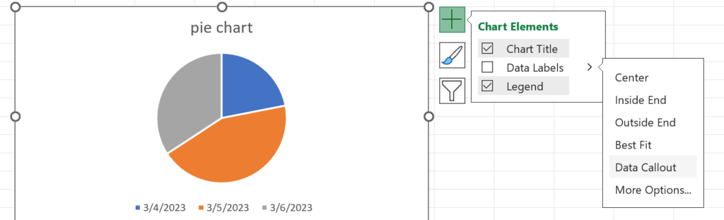
2.1342.Click on”More Options”.
3.Uncheck the “Percentage” box
Q61.Change the chart title of the pie chart to “Percentage of sales by day”.
answer
1.Click on the chart title of a pie chart to delete the text string.
*Be careful not to delete an entire element; delete it while the text cursor(the vertical bar that blinks when you type text) is displayed, as shown in the image.
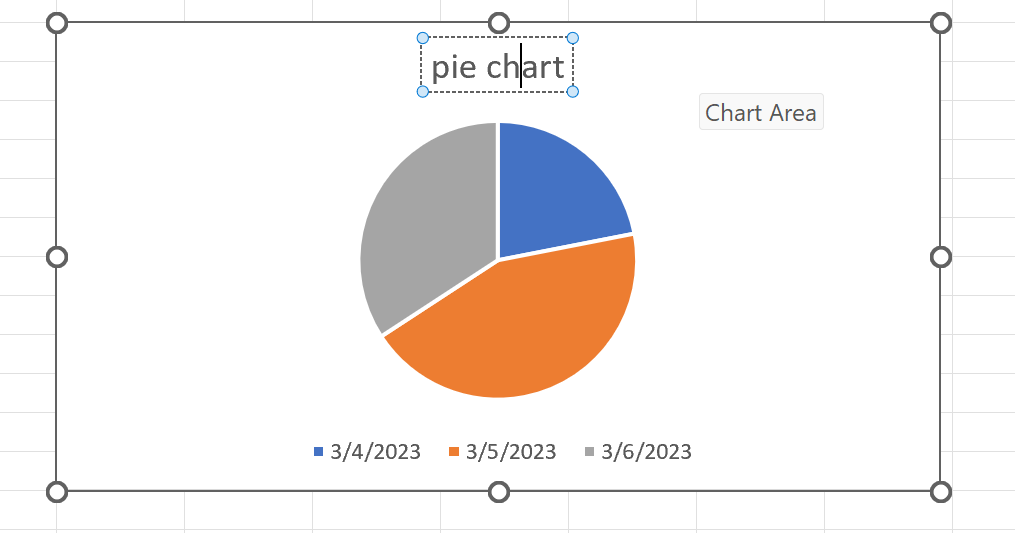
2.Copy and paste”Percentage of sales per day”from the question.
To confirm a value, click outside the graph.
(Advance preparation)
Use the DailySales table to create the below line chart.
1.Select everything except for the total from the Daily Sales table.
2.Insert tab-click on”Recommended Charts” in Charts.
3.Select “Line Chart” and click”OK.
Q62.Apply “Layout 1” to the line chart.
answer
1.Select a line chart and click on the”Chart Design”tab-“Quick Layout.

2.Select “Layout 1” from the suggestions.
*Place the mouse pointer over it to see the name
Q63.Move the line chart to the Chart sheet named “Sales Trend Analysis Chart”.
answer
1.Select the line chart, then click on the Chart Design tab-Move Chart.
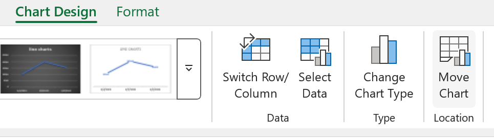
2.Choose a new sheet, copy and paste “Sales Trend Analysis Chart” from the question into the sheet name, and click [OK].
(Advance preparation)
Create the below table.
Q64.Using the table “Test results”, create a Clustered bar chart showing totals by name.
answer
1.Select the name and total columns of the table (select the Name column, then hold down Ctrl and select the total amount column).
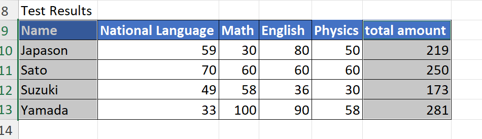
2.Insert tab-click on “RecommendedCharts” in Charts.
3.Select “Clustered Bar”.
(Advance preparation)
Using the table “Test results”, create a Clustered column chart.
1.Select everything except total column of the table.
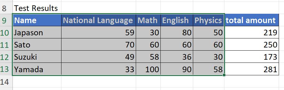
2.Insert tab-click on”Recommended Charts” in Charts.
3.Select “Clustered column chart ” and click”OK.
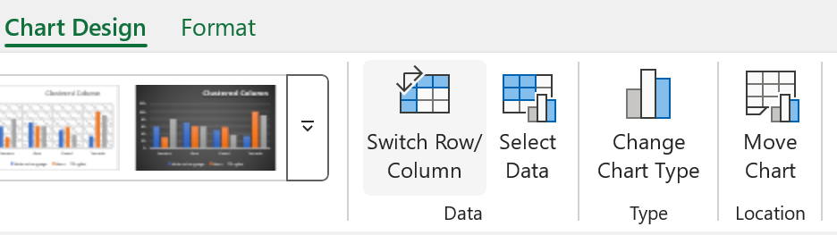
Q65.Switch the horizontal axis and the legend of the Clustered Column chart to display subjects on the horizontal axis and names on the legend.
answer
1.Select the Clustered Column chart and click on the Chart Design tab-SwitchRow/Column.
Q66.Place the created chart in the cell range A20:H33.
answer
1.While holding down the Alt key, move the graph to align it with the upper left corner of cell A20.
2.Hold down the Alt key and enlarge the right side of the chart to align with the right side of column H.
3.Hold down the Alt key and enlarge the bottom of the chart to align with the bottom of line 33.
(Advance preparation)
Using the table “Test results”, create a Vertical stacked bar chart choosing only Japanese, Mathematics, and English.
1.Select everything except total and physics columns of the table.
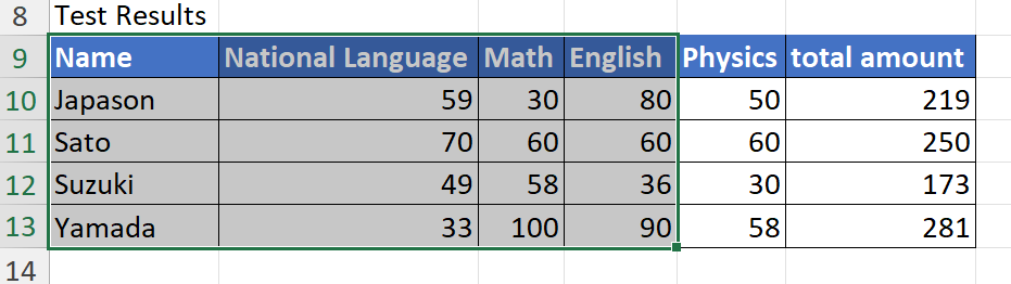
2.Insert tab-click on”Recommended Charts” in Charts.
3.Select “Vertical stacked bar chart ” and click”OK.
Q67.Add a data series of physics to the Vertical stacked bar chart.
answer
1.Select a Vertical stacked bar chart.
2.Drag the blue box to the right to include physics in the data range of the table.
Q68.Apply the style “Style 6” and the color “Monochromatic Palette1” to the Vertical stacked bar chart.
answer
1.Select the Vertical stacked bar chart, then select ChartDesign tab-ChartStyles, 6th one from the left.
2.From the Design tab-Change Colors, select Monochromatic Palette.
Q69.Set the alternative text “Score Chart by Student” for the Vertical stacked bar chart.
answer
1.Right-click on the Vertical stacked bar chart and click View Alt text.
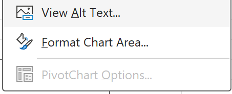
2.Copy and paste the “Score Chart by Student” from the question.
MO-210:Pass With 91 Questions
if you can solve all the questions in this video, you will definitely pass the exam.